
Earth Scientists focus on today’s pressing challenges to society: earthquake risk, sustainability, water resources, ocean health, natural resources and societal impact of changing climate/atmospheric chemistry. We also tackle the foremost problems in the earth sciences: the temporal and spatial evolution of life, habitability, the origin and movement of Earth’s crust, deep earth structure and the study of complex chemical cycles.
USC Earth Sciences in the field

@drjoshwest
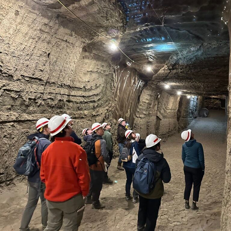
Fantastic start to our @USC_earth @USCDornsife #Alaska field class at the Army Corps Permafrost Research Tunnel, exploring frozen ground, ancient grasses, ice wedges, and mammoth bones… oh and the pungent smell of permafrost! Huge thanks to @USACEHQ CRREL for hosting us!

@drjoshwest
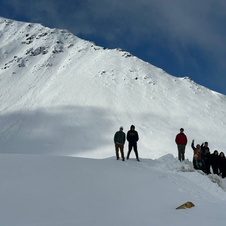
Incredible #aufeis on the North Slope of Alaska near @Toolik with @USC_earth field class. These seasonal accumulations of layered ice form in the Arctic where ground water discharges and successfully freezes, building up then eroding from underneath during Spring thaw. Amazing!
Exciting 2 days w/ @USC_earth field class on fabled Dalton Hwy. Trucks servicing Alaska’s oil fields make 414-mile gravel road an adventure but also amazing opportunity to reach remote tundra off the North Slope. Pipeline, Arctic Circle, & caribou herds just some highlights.
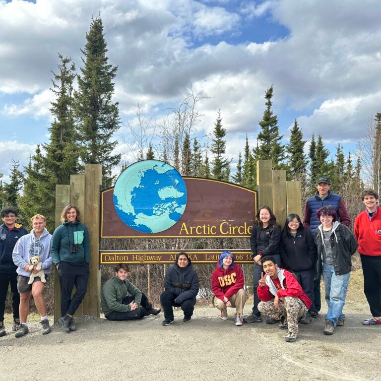
Exciting 2 days w/@USC_earth field class on fabled Dalton Hwy. Trucks servicing Alaska’s oil fields make 414-mile gravel road an adventure but also amazing opportunity to reach remote tundra of the North Slope. Pipeline, Arctic Circle, & caribou herds just some highlights.
Amazing ancient ice wedge features come to life in the USACE permafrost tunnel. White ice filled in voids where older brown ice melted. Ice wedges warped surrounding layers as they formed and expanded. Amazing opportunity to be able to take our @USC_earth class there.
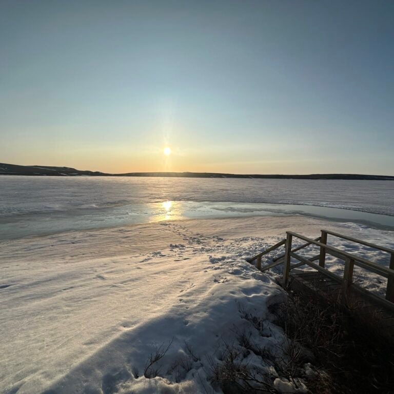
Had fantastic opportunity to spend 5 days
@Toolik Field Station in #Arctic of northern Alaska with @USC_earth class. Thanks to everyone at this amazing facility for allowing us to explore tundra & learn water chemistry in this rapidly changing environment. It’ll be hard to leave!
Global Impact


Looking for PhD Students!
Professors Will Berelson and Josh West are looking for PhD students interested the following topics:
Urban Trees and Air Quality
Urban Trees and Hydrology
The Urban Critical Zone and urban carbon cycle
We have several projects in mind and RA support for a student versed in geo/bio sciences with desire to conduct chemistry and field work. Familiarity with gas measurements desirable. Potential to expand into atmospheric modeling and AI work. But primary effort would be to join a team of geochemists, embedded in a team which includes urban landscape architects and GIS specialists to address the values, costs, benefits of urban vegetation and hardscape. Because your degree would be in Earth Sciences, those who interests aligned most closely with earth system research would be most highly regarded.

USC Earth Sciences at a Glance
50+
Graduate Students
20+
Full Time Faculty
10+
Research and Adjunct Faculty
28th
Earth Sciences graduate program rankings, US News 2022
21+ million
Research Funding
Contact Us
Main Office
Department of Earth Sciences
Zumberge Hall of Science (ZHS)
3651 Trousdale Pkwy
Los Angeles, CA 90089-0740